

Repository
glm-5.2-in-c
GLM-5.2, a 744 billion parameter mixture of experts model, in a pure C inference engine: quantized to int4, experts streamed from disk, deployed and benchmarked. Generates in 16 GB of RAM.
README
Building GLM 5.2 in C to Run a 744B Model on Consumer Hardware
Quantize it to int4, stream the experts from disk, and serve it from one machine
About this repository. What follows is the complete write-up. The repository also holds the pure C engine, the deployment automation, the benchmark harness, and every measurement referenced below. If you would rather build and run it first, jump to Get the code and build. The engine and the conversion tools are derived from the colibri project by JustVugg, under the Apache License 2.0 (see NOTICE). The original work in this repository is the restructuring, the documentation, the cloud deployment, the benchmark harness, the measurement corpus under
results/, and the analysis.
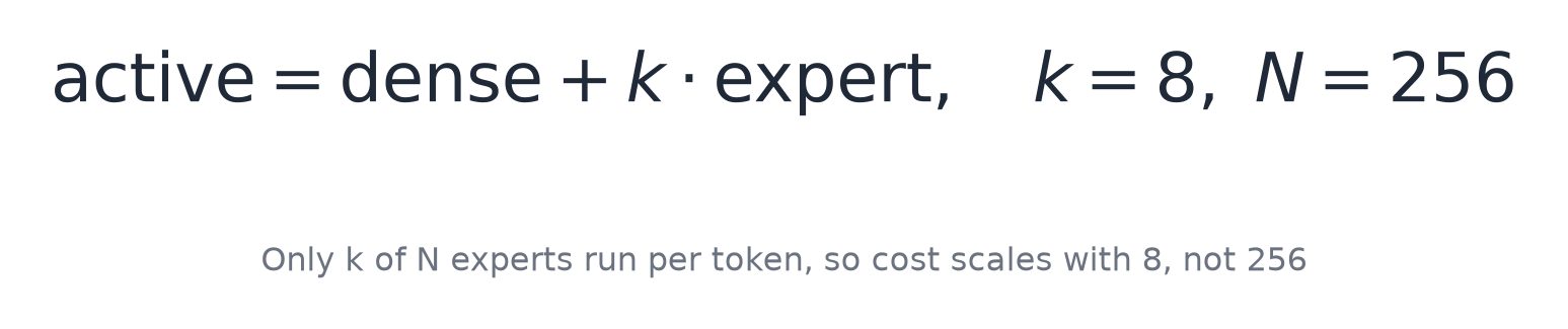
GLM 5.2 is a 744 billion parameter model, about 1.5 terabytes in bfloat16, and the usual way to run something that big is a rack of datacenter GPUs. But it is a Mixture of Experts, so only 8 of its 256 experts per layer fire for any given token, and most of the model sits asleep. If we keep the small always on part in memory and stream the sleeping experts from disk, the working set stays tiny even though the model on disk is enormous. So it can fit on a laptop with about 16 gigabytes of RAM and no GPU, running an engine we build from scratch in pure C.

Here is everything we build, all in one C file with no BLAS and no framework, top to bottom, one component at a time:
- Set up and build: inspect the box and the model, then compile the engine from a single C file into a 377 kilobyte binary.
- Prove the idea small first: a 400 line streaming engine for a smaller model, validated token for token against PyTorch.
- Quantize FP8 to int4: dequantize the vendor weights and repack them to 4 bits with per row scales, and measure what that costs.
- Load weights by streaming: index and read tensors on demand with
pread, and drop the pages right after. - Run the forward pass: multi head latent attention with a compressed KV cache, a sparse attention indexer, and the Mixture of Experts router.
- Write the kernels: integer dot products for int4 and int8 weights, checked bit for bit against a plain C reference.
- Build the tiering system: place experts across VRAM, pinned RAM, an LRU cache, the page cache, and disk, then prefetch and pipeline so compute overlaps the reads and it never runs out of memory.
- Speculate: draft tokens with the model's own multi token head, with n grams, and with a grammar, then verify them losslessly.
- Serve it: an OpenAI compatible server with a proper scheduler, streaming, and backpressure.
- Prove it works: actual conversations, the full performance story, and the correctness checks that got us here.
Every number and every log line in this post comes from runs on our own hardware. All of the code is available in my GitHub repository (theory plus code): GitHub repo for the GLM 5.2 C engine.
The codebase is organized as follows.
glm-5.2-in-c/
├── engine/                     # the C engine
│   ├── glm.c                   # the whole engine in one file
│   ├── st.h, tier.h            # streaming loader and expert tiering
│   ├── olmoe.c                 # the 400 line stepping stone we build first
│   ├── backend_cuda.cu         # optional CUDA kernels
│   └── Makefile                # one command builds it
├── tools/                      # offline Python
│   ├── convert_fp8_to_int4.py  # the FP8 to int4 requantizer
│   └── make_glm_oracle.py      # the tiny PyTorch reference we validate against
├── cli/                        # entry point and server
│   └── openai_server.py        # the OpenAI compatible API
├── docs/                       # the longer theory write ups
├── results/                    # every log and number quoted in this post
├── deploy/                     # provisioning and run scripts
└── bench/                      # the capture scripts behind the results
So let us get started and build it up, one piece at a time.
Why a 744B Model Can Fit
The problem is not "buy more GPUs." It is to stop pretending you need all 744 billion parameters at once. A Mixture of Experts model has a router that, for each token, picks a few experts and ignores the rest.

Let me put some numbers on this. GLM 5.2 has 78 layers, the first 3 dense and the other 75 with 256 experts each. The router picks the top 8 per token, so only about 3 percent of the experts fire.
That sparsity is the point. The always on part is about 17 billion parameters, or 9.9 gigabytes at 4 bits, and it stays in RAM. The routed experts are the other 727 billion, about 362 gigabytes on disk.
And only 8 experts per layer change from one token to the next. So of that 362 gigabytes, only about 11 gigabytes are touched per token, mostly the same hot experts over and over.
Now for the size of one expert. Its weight is an O by I matrix, and at 4 bits we pack two values per byte, so it is O times ceil(I/2) bytes plus one scale per row.
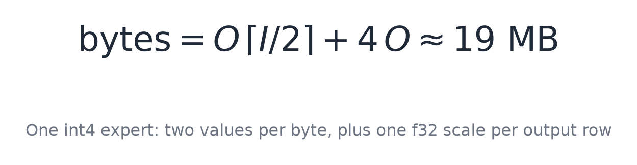
For GLM 5.2 that is three matrices, gate, up, and down, about 19 megabytes per expert. That 19 megabyte read is the unit of work, and the whole post is about making it cheap, cached, or skipped.
The Model, and the Hardware It Runs On
Before writing a line of the engine, let us look at what we are running and what it actually asks of a machine. The surprising part is how little it asks, and that is the whole reason this fits on hardware you own.
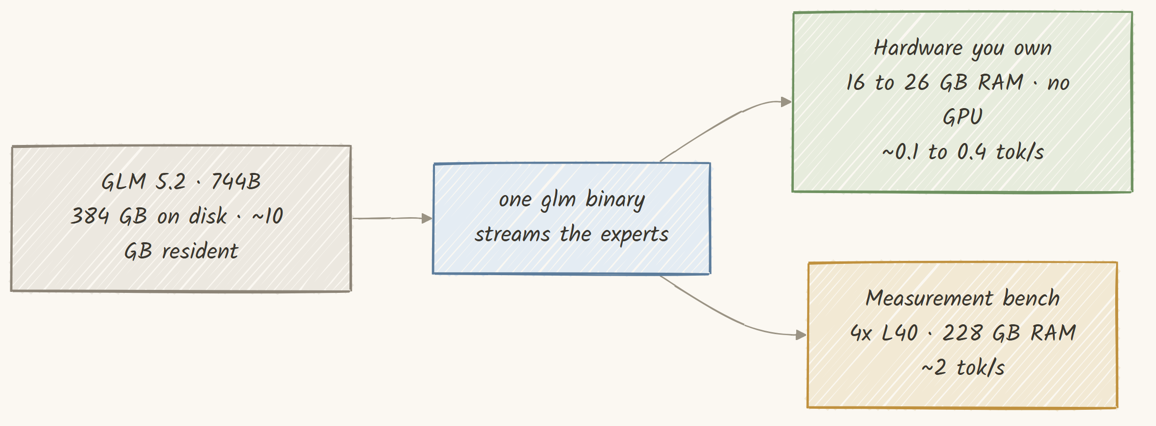
As we just saw, only about 10 gigabytes of this model ever needs to stay resident, and the rest streams from disk on demand.
So the floor is not a datacenter. It is a normal machine with a normal amount of RAM and a fast enough disk.
Here is that floor, the machine this is for.
The floor: a machine you already own
CPU     any modern x86-64 (AVX2 helps) or Apple Silicon
RAM     about 16 to 26 GB
disk    an NVMe SSD with room for the int4 model
GPU     none required
This is not aspirational. People run this exact 744 billion parameter model in pure C, with the experts streamed from disk, on a Framework 13 laptop at about 0.37 tokens per second and on a desktop at around 0.1 to 0.3.
I will show the full spread of machines at the end. The point for now is that no GPU and no server appears in that list.
So why does the rest of this post talk about a much bigger box? Because we do our measuring on one, and I would rather be plain about that than hide it.
Our development bench is a single workstation with 4 NVIDIA L40 GPUs, an AMD EPYC 7763 CPU, 228 gigabytes of RAM, and a 3.2 terabyte NVMe drive. We use it because it gives clean, repeatable numbers, and because it lets us show what headroom buys, not because you need it.
Here is its CPU and memory picture, captured with lscpu and free.
Model name:            AMD EPYC 7763 64-Core Processor
CPU(s):                124
Thread(s) per core:    1
Core(s) per socket:    62
Socket(s):             2
NUMA node(s):          2
L3 cache:              1.9 GiB

CPU AVX flags (note: AVX2 present, NO avx512/vnni)
avx avx2 fma sse4_1 sse4_2

               total        used        free      shared  buff/cache   available
Mem:           228Gi       136Gi       2.9Gi        51Mi        90Gi        91Gi
Swap:             0B          0B          0B
The one line I want you to notice is the AVX flags. This CPU has AVX2 and FMA, but it does not have AVX-512 or the VNNI integer dot instructions. That matters a lot later, because our fastest integer kernels would love VNNI, and we will have to fall back to AVX2 and measure what we actually get.
Writing the number down now saves confusion when the kernel section arrives.
Here are the 4 GPUs, from nvidia-smi.
NVIDIA-SMI 570.195.03   Driver Version: 570.195.03   CUDA Version: 12.8
GPU  Name          Memory-Usage         GPU-Util
  0  NVIDIA L40    44543MiB / 49140MiB      0%
  1  NVIDIA L40    44543MiB / 49140MiB      0%
  2  NVIDIA L40    44545MiB / 49140MiB      0%
  3  NVIDIA L40    44543MiB / 49140MiB      0%
Four L40 cards, about 49 gigabytes each, for a total of roughly 196 gigabytes of VRAM. Notice they are already 44.5 gigabytes full and the utilization is 0 percent. That is the engine at rest with experts pinned into VRAM, a luxury this bench has and the floor does not. On a machine with no GPU the same binary simply streams those experts from RAM and disk instead. We will get to how they got there.
So we run the experiments on this bigger box because it is faster to analyze and test, but everything it does the cheapest machine does too, only slower.
The entire software dependency surface is three tools.
gcc (Ubuntu 13.3.0-6ubuntu2~24.04.1) 13.3.0
nvcc: Cuda compilation tools, release 12.8, V12.8.93
Python 3.12.3
A C compiler for the engine, nvcc for the optional GPU backend, and Python only for the offline weight conversion. The running engine imports none of them. Now the model itself. The architecture lives in config.json, and these are the fields that shape everything we write.
{
  "architectures": ["GlmMoeDsaForCausalLM"],
  "model_type": "glm_moe_dsa",
  "hidden_size": 6144,
  "num_hidden_layers": 78,
  "first_k_dense_replace": 3,
  "num_attention_heads": 64,
  "num_key_value_heads": 64,
  "n_routed_experts": 256,
  "num_experts_per_tok": 8,
  "n_shared_experts": 1,
  "moe_intermediate_size": 2048,
  "q_lora_rank": 2048,
  "kv_lora_rank": 512,
  "qk_nope_head_dim": 192,
  "qk_rope_head_dim": 64,
  "v_head_dim": 256,
  "index_head_dim": 128,
  "index_n_heads": 32,
  "index_topk": 2048,
  "num_nextn_predict_layers": 1,
  "vocab_size": 154880,
  "scoring_func": "sigmoid",
  "topk_method": "noaux_tc",
  "routed_scaling_factor": 2.5,
  "rope_parameters": { "rope_theta": 8000000 },
  "quantization_config": {
    "quant_method": "fp8", "fmt": "e4m3", "weight_block_size": [128, 128]
  }
}
There is a lot here, and we will meet each field when it matters. For now, the shape of the model is hidden size 6144, 78 layers with the first 3 dense, 256 experts per layer with top 8 routing, and one shared expert.
The attention is Multi head Latent Attention, which is the q_lora_rank, kv_lora_rank, and the split qk_nope and qk_rope head dims. There is a sparse attention indexer with index_topk of 2048. There is a multi token prediction head.
And the last field is the important one for the next section: the vendor ships this model in FP8, in the e4m3 format, with 128 by 128 block scales.
When we run our own small status tool, it reads the config and the machine and prints a one screen summary, a quick sanity check that everything lines up.
model      /nvme/glm52_i4
arch       hidden 6144 · 78 layer · 256 expert/layer · top-8
shards     144 files · 384 GB on disk
RAM        239 GB total · 232.6 GB available
disk       3029 GB free
engine     ready
So the model is 384 gigabytes on disk across 144 shards, and the bench has plenty of RAM to spare. This status tool prints the total as 239 gigabytes where free rounds it to 228, but either way the model itself needs only about 10 gigabytes resident, so the rest is headroom for caching hot experts. Note the directory name, glm52_i4. That i4 is int4, our own 4 bit conversion of the vendor's FP8 weights. We will build that conversion ourselves in a couple of sections.
Building the Engine, One C File With No BLAS
The engine is a single C translation unit, glm.c, of about 3,900 lines, plus a handful of header only helpers. There is no BLAS, no framework, and nothing to link except the math library and OpenMP.
I like this because it means the whole thing compiles in a second and the binary is small enough to read the disassembly if you ever need to.
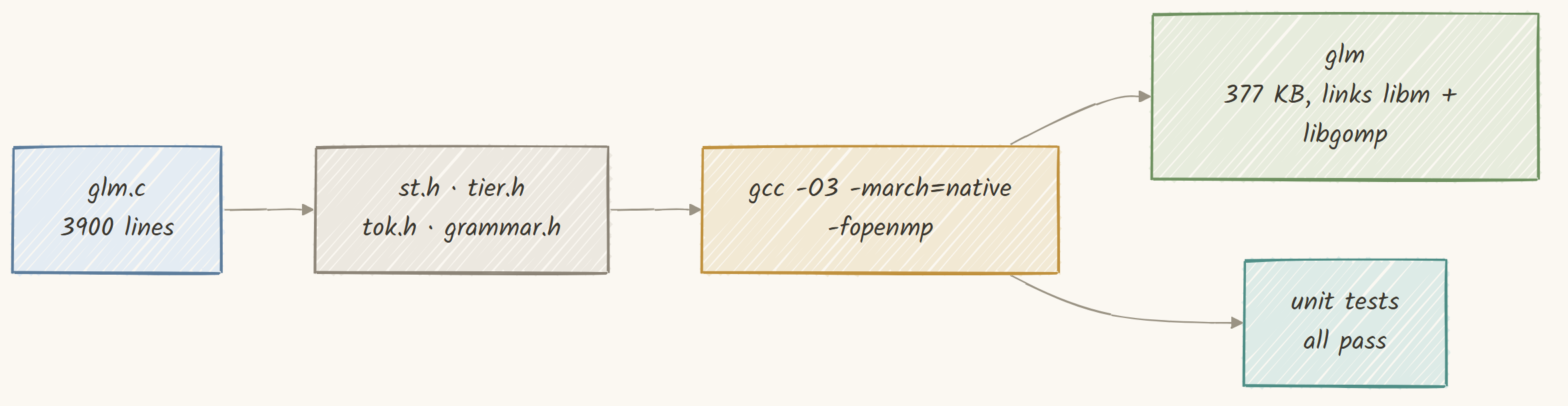
Building for CPU is one command, and here is the exact line the build runs.
gcc -O3 -march=native -fopenmp -Wall -Wextra glm.c -o glm -lm -fopenmpThat is the whole CPU build. -O3 for optimization, -march=native so the compiler uses the AVX2 and FMA our CPU has, and -fopenmp for the thread parallelism inside our matmuls. It links libm and libgomp and nothing else.
If we want the optional GPU backend, we compile one extra CUDA file and link the CUDA runtime.
nvcc -O3 -std=c++17 -arch=sm_89 -c backend_cuda.cu -o backend_cuda.o
gcc -O3 -march=native -fopenmp -DGLM_CUDA glm.c backend_cuda.o -o glm -lm -fopenmp \
    -L/usr/local/cuda/lib64 -lcudart -lstdc++
The GPU is strictly optional. The -DGLM_CUDA define is the only thing that pulls in the CUDA path, and -arch=sm_89 targets the Ada architecture of the L40. If you never pass that define, you get a pure CPU engine that runs on a laptop.
Let me show you how small the result is.
-rwxrwxr-x 1 ubuntu ubuntu 376648 Jul 14 06:37 glmThe whole engine is a 376,648 byte binary, about 377 kilobytes. A 744 billion parameter model driven by a 377 kilobyte program.
We also have a set of unit tests, and every one of them is built and run on its own so a failure is easy to localize. Let us run them and see.
----- test_json -----          json tests: ok
----- test_st -----            safetensors primitive tests: ok
----- test_tier -----          tier tests: ok
----- test_grammar -----       test_grammar: ok
----- test_decode_batch -----  decode batch helper tests: ok
----- test_idot -----          idot kernel exactness (avx2): ok
----- test_i4_acc512 -----     test_i4_acc512: skipped (no AVX-512 on this build)
Everything passes, and one test is deliberately skipped. The test_i4_acc512 test checks an AVX-512 kernel, and this EPYC has no AVX-512, so the test skips instead of pretending.
The headline line for me is idot kernel exactness (avx2): ok, which is the proof that our hand written AVX2 integer dot product matches a plain C reference bit for bit. We will look at that kernel later.
One small but important detail about the build and the runtime. The per expert matmuls are tiny and back to back, and with OpenMP's default passive wait policy the worker threads get parked between regions and the wake up latency dominates.
The engine fixes this by setting the OpenMP thread policy to active spin and then re executing itself once so a fresh OpenMP runtime picks up the setting. On the Zen build this took the matmul time from 66.9 seconds down to 20.9 seconds with no change to the output.
It is the kind of thing you only find by measuring, and you see it in the logs as a one line notice at startup.
[OMP] hot-thread tuning: re-exec once (GLM_NO_OMP_TUNE=1 to skip)The Math Primitives, Written by Hand
Before the big components, let us start with the small ones, because the whole engine stands on a handful of tiny math functions that we wrote ourselves. There is no library underneath, so every normalization, every activation, and the rotary position embedding is a few lines of C.
The first is RMS normalization, which the model applies before attention and before the feed forward. It divides each vector by the root mean square of its own elements, then scales by a learned weight.
/* RMS norm: divide by the root-mean-square of the vector, then scale by w. */
static void rmsnorm(float *out, const float *x, const float *w, int D, float eps) {
    double ms = 0; for (int i = 0; i < D; i++) ms += (double)x[i] * x[i];
    float r = 1.f / sqrtf((float)(ms / D) + eps);
    for (int i = 0; i < D; i++) out[i] = x[i] * r * w[i];
}
We accumulate the sum of squares in a double, not a float, because a 6144 element vector loses precision if you add thousands of squares in single precision, and that precision is part of what lets us match the reference exactly. The next two are the softmax and the SiLU activation.
/* Softmax, shifted by the max for numerical stability. */
static void softmax(float *x, int n) {
    float m = -1e30f; for (int i = 0; i < n; i++) if (x[i] > m) m = x[i];
    float s = 0; for (int i = 0; i < n; i++) { x[i] = expf(x[i] - m); s += x[i]; }
    for (int i = 0; i < n; i++) x[i] /= s;
}
/* SiLU, the activation inside every SwiGLU expert. */
static inline float siluf(float x) { return x / (1.f + expf(-x)); }
The softmax subtracts the maximum before it exponentiates, which is the standard way to avoid overflow. SiLU is one line. The last primitive is the rotary position embedding, which rotates pairs of query and key elements by an angle that grows with the token's position, so attention can tell where each token sits.
/* Rotary position embedding, interleaved. Each pair (2j, 2j+1) is rotated by an
 * angle that grows with the position, so attention becomes position-aware. */
static void rope_interleave(float *v, int pos, const Cfg *c) {
    int half = c->qk_rope / 2; float in[256]; memcpy(in, v, c->qk_rope * sizeof(float));
    for (int j = 0; j < half; j++) {
        float inv = powf(c->theta, -2.0f * j / c->qk_rope);
        float ang = pos * inv, cs = cosf(ang), sn = sinf(ang);
        float a = in[2*j], b = in[2*j + 1];
        v[j]        = a * cs - b * sn;
        v[half + j] = b * cs + a * sn;
    }
}
These few functions, plus the matmuls, are enough to assemble one transformer layer. A layer is a norm, then attention, then a residual add, then another norm, then the Mixture of Experts, or a dense feed forward for the first three layers, then another residual add. Here is exactly that, from the layer driver.
/* One layer: in_norm -> attention -> residual -> post_norm -> MoE/dense -> residual. */
for (int s = 0; s < S; s++) rmsnorm(nrm + (int64_t)s*D, x + (int64_t)s*D, l->in_ln, D, c->eps);
attention_rows(m, l, li, nrm, S, pos_base, kvs, positions, tmp);
for (int64_t j = 0; j < (int64_t)S*D; j++) x[j] += tmp[j];                 /* residual */
for (int s = 0; s < S; s++) rmsnorm(nrm + (int64_t)s*D, x + (int64_t)s*D, l->post_ln, D, c->eps);
if (l->sparse) moe(m, l, li, nrm, S, tmp);
else dense_mlp(l, nrm, S, D, c->dense_inter, tmp);
for (int64_t j = 0; j < (int64_t)S*D; j++) x[j] += tmp[j];                 /* residual */
Run that for all 78 layers, take the last position's hidden state, normalize it one more time, and multiply by the output embedding to get the logits over the vocabulary. That loop, wrapped around the components we are about to build, is the entire forward pass.
Everything else in this post is about making each of those steps fit in memory and run fast.
First, the Streaming Idea in 400 Lines
Before we take on the full 3,900 line engine for GLM 5.2, I want to prove the idea on something smaller and simpler. The idea is "keep the dense part resident, stream the experts from disk," and we can show it works in about 400 lines of C for a smaller Mixture of Experts model.
This smaller engine is olmoe.c, and its only job was to reproduce the exact token ids of a reference before we scaled up. If the streaming approach is correct here, we can trust it when we make it complicated.

The key part is how we hold an expert in memory. We do not keep experts as full precision floats, because that would defeat the purpose. We keep each weight matrix as int8, one byte per parameter, with one float scale per row.
That already takes the RAM cost from 4 bytes per parameter down to 1, and we dequantize on the fly inside the matmul. Here is the cache slot.
/* One expert's weights, held quantized. Each matrix [out,in] is int8 per row
 * plus one float scale per row. This is what takes the RAM cost from
 * 4 bytes/param (f32) down to 1 byte/param. We dequantize on use in the matmul. */
typedef struct { int eid; int8_t *g, *u, *d; float *gs, *us, *ds; uint64_t used; } Slot;
typedef struct { Slot *slots; int n, cap; } LCache;
The Slot holds the three matrices of one expert, gate, up, and down, as int8 buffers, plus their per row scales, plus a used counter for least recently used eviction. The LCache is just an array of these slots, one cache per layer. Now the quantizer that fills those buffers.
It is symmetric and per row, which means for each output row we find the largest absolute value, divide it by the maximum representable integer to get a scale, and store the rounded quotient.
/* Quantize a weight [O,I] to int8 q[O,I] plus a per-row scale, symmetric.
 * scale = max(|w|, over the row) / qmax, and q = round(w/scale). */
static void quantize_rows(const float *w, int8_t *q, float *scale, int O, int I, int bits) {
    int qmax = (1 << (bits - 1)) - 1;     /* 8 bits -> 127, 4 bits -> 7 */
    #pragma omp parallel for schedule(static)
    for (int o = 0; o < O; o++) {
        const float *wr = w + (int64_t)o * I;
        float amax = 0.f;
        for (int i = 0; i < I; i++) { float a = fabsf(wr[i]); if (a > amax) amax = a; }
        float s = amax / qmax; if (s < 1e-8f) s = 1e-8f;
        scale[o] = s;
        int8_t *qr = q + (int64_t)o * I;
        for (int i = 0; i < I; i++) {
            int v = (int)lrintf(wr[i] / s);
            if (v >  qmax) v =  qmax;
            if (v < -qmax - 1) v = -qmax - 1;
            qr[i] = (int8_t)v;
        }
    }
}
This is the exact quantization math we will reuse for the big model too, so it is worth reading carefully. Each row gets its own scale from its own maximum absolute value, we round to the nearest integer with lrintf, and we clamp into the int8 range. There is nothing clever here, and that is the point.
Simple, per row, symmetric quantization is enough to keep the model working, as we will confirm with numbers.
Now the streaming itself. When the router asks for an expert, we look it up in the per layer cache. If it is there, that is a hit and we bump its recency.
If it is not, that is a miss, and we either grow the cache or evict the least recently used slot, then read the three matrices from disk and quantize them into the slot.
/* Return the quantized weights of one expert, from cache or from disk.
 * A hit bumps recency. A miss evicts the least-recently-used slot, then
 * reads the three matrices from disk and quantizes them into it. */
static void expert_get(Model *m, int layer, int eid, Slot **out) {
    LCache *lc = &m->cache[layer];
    for (int i = 0; i < lc->n; i++) if (lc->slots[i].eid == eid) {
        m->hits++; lc->slots[i].used = ++m->clock; *out = &lc->slots[i]; return;
    }
    m->miss++;
    Slot *s;
    if (lc->n < lc->cap) {                       /* room: grow the cache */
        s = &lc->slots[lc->n++];
        s->g = malloc(ng); s->u = malloc(ng); s->d = malloc(nd);
        s->gs = falloc(c->inter); s->us = falloc(c->inter); s->ds = falloc(c->hidden);
    } else {                                     /* full: evict the LRU slot */
        int lru = 0;
        for (int i = 1; i < lc->n; i++) if (lc->slots[i].used < lc->slots[lru].used) lru = i;
        s = &lc->slots[lru];
    }
    /* read gate, up, down from disk (pread + fadvise DONTNEED), quantize into the slot */
    load_expert_w(m, gate_name, s->g, s->gs, c->inter, c->hidden, tmp);
    load_expert_w(m, up_name,   s->u, s->us, c->inter, c->hidden, tmp);
    load_expert_w(m, down_name, s->d, s->ds, c->hidden, c->inter, tmp);
    s->eid = eid; s->used = ++m->clock;
    *out = s;
}
The hits and miss counters are how we will measure whether the cache is doing its job. And then the Mixture of Experts step ties it together. For each token, we run the router, take the top k experts, and for each one we fetch it from the cache, run the SwiGLU feed forward, and add its weighted contribution.
/* The MoE step for tokens x[S,hidden] -> out[S,hidden]. Route, take top-k,
 * fetch each expert from cache, run its SwiGLU, add its weighted output. */
static void moe(Model *m, Layer *l, int layer, float *x, int S, float *out) {
    Cfg *c = &m->c; int D = c->hidden, E = c->n_experts, K = c->topk, I = c->inter;
    float *logits = falloc((int64_t)S * E);
    matmul(logits, x, l->gate, S, D, E);
    memset(out, 0, (int64_t)S * D * sizeof(float));
    for (int s = 0; s < S; s++) {
        float *pr = logits + (int64_t)s * E;
        softmax_row(pr, E);
        int idx[64]; float val[64];                  /* pick the top-K experts */
        for (int kk = 0; kk < K; kk++) {
            int best = -1; float bv = -1e30f;
            for (int e = 0; e < E; e++) {
                int taken = 0; for (int j = 0; j < kk; j++) if (idx[j] == e) { taken = 1; break; }
                if (!taken && pr[e] > bv) { bv = pr[e]; best = e; }
            }
            idx[kk] = best; val[kk] = bv;
        }
        const float *xs = x + (int64_t)s * D;
        for (int kk = 0; kk < K; kk++) {
            Slot *e; expert_get(m, layer, idx[kk], &e);            /* cache or disk */
            matmul_q(g, xs, e->g, e->gs, D, I);                   /* gate_proj */
            matmul_q(u, xs, e->u, e->us, D, I);                   /* up_proj   */
            for (int i = 0; i < I; i++) { float gv = g[i]; g[i] = (gv / (1.f + expf(-gv))) * u[i]; }
            matmul_q(hh, g, e->d, e->ds, I, D);                   /* down_proj */
            float w = val[kk];
            float *os = out + (int64_t)s * D;
            for (int d = 0; d < D; d++) os[d] += w * hh[d];       /* weighted add */
        }
    }
}
Read this and the big model's Mixture of Experts step will feel familiar, because it is the same shape, only with more machinery bolted on. Route, select, fetch from cache or disk, run a SwiGLU, add. When we run this small engine against its reference, it matches token for token.
== Streaming C engine, cache = 16 experts/layer, experts @ 8-bit ==
resident weights loaded in ... | RSS after load: ... GB

Reference: 207 187 119 103 103 103 103 103 119 34 ...
C engine : 207 187 119 103 103 103 103 103 119 34 ...
Matching tokens: 20/20
Expert cache hit rate: ...  (hit=... miss=...)
Twenty out of twenty tokens match the reference. That is the whole reason olmoe.c exists. It is the small, solid proof that a dense resident, expert streaming engine can be exactly correct, not just approximately. Now we can scale the idea up to the full model with confidence.
Quantization: From FP8 to int4
The vendor ships GLM 5.2 in FP8. That is a floating point format with an 8 bit exponent and mantissa layout called e4m3, and the checkpoint is about 756 gigabytes. Two problems with running it as is.
First, a normal CPU cannot do arithmetic in e4m3, there is no instruction for it, so we would spend all our time converting. Second, 756 gigabytes is a lot to keep and move.
So we do our own offline conversion, from FP8 to int4 with per row scales, which halves the bytes and gives us a format that integer SIMD can use directly.

The quantization math is the same symmetric per row absmax we used in the small engine, and it must be identical to what the C engine expects, byte for byte, or the tokens will not match. Here is the scale and rounding.
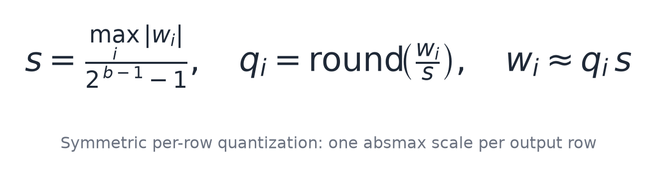
The int4 case adds packing. Each quantized value fits in a nibble in the range from negative 8 to positive 7, and we store two nibbles per byte.
To keep the bytes unsigned we store each value plus 8, so the range becomes 0 to 15, and the low nibble is the first value while the high nibble is the second value shifted up by 4.
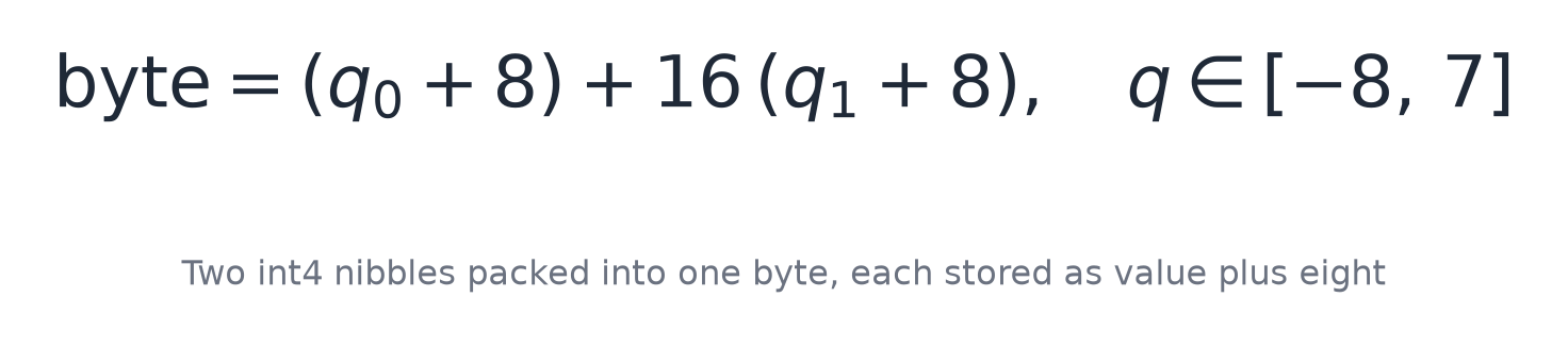
Here is the converter's int4 packer. It is NumPy, and every line has a mirror in the C engine.
def quant_int4(w, bits):                        # w: [O,I] f32 -> (U8 bytes, f32 scale [O])
    O, I = w.shape
    qmax = (1 << (bits - 1)) - 1
    amax = np.abs(w).max(axis=1, keepdims=True)          # per-row absmax
    s = np.maximum(amax / qmax, 1e-8)                    # per-row scale
    q = np.clip(np.rint(w / s), -8, qmax).astype(np.int32)   # nibble in [-8, 7]
    rb = (I + 1) // 2
    out = np.zeros((O, rb), np.uint8)
    v0 = (q[:, 0::2] + 8).astype(np.uint8)               # even values -> low nibble
    out[:, :v0.shape[1]] = v0
    if I > 1:
        v1 = (q[:, 1::2] + 8).astype(np.uint8)           # odd values -> high nibble
        out[:, :v1.shape[1]] |= (v1 << 4)
    return out.reshape(-1), s[:, 0].astype(np.float32)
And here is the C engine's packer, from glm.c. Look at the last line of the inner loop and compare it to the NumPy above.
/* Pack w[O,I] f32 -> int4 (2 per byte) + a per-row scale.
 * Values in [-8,7] are stored as v+8 (0..15), low nibble then high nibble. */
static void pack_int4(const float *w, uint8_t *q4, float *scale, int O, int I, int bits) {
    int qmax = (1 << (bits - 1)) - 1, rb = (I + 1) / 2;
    #pragma omp parallel for schedule(static)
    for (int o = 0; o < O; o++) {
        const float *wr = w + (int64_t)o * I; float amax = 0;
        for (int i = 0; i < I; i++) { float a = fabsf(wr[i]); if (a > amax) amax = a; }
        float s = amax / qmax; if (s < 1e-8f) s = 1e-8f; scale[o] = s;
        uint8_t *qr = q4 + (int64_t)o * rb;
        for (int i = 0; i < I; i += 2) {
            int v0 = (int)lrintf(wr[i] / s); if (v0 > qmax) v0 = qmax; if (v0 < -8) v0 = -8;
            int v1 = 0; if (i + 1 < I) { v1 = (int)lrintf(wr[i+1] / s); if (v1 > qmax) v1 = qmax; if (v1 < -8) v1 = -8; }
            qr[i >> 1] = (uint8_t)((v0 + 8) | ((v1 + 8) << 4));
        }
    }
}
The Python uses np.rint and the C uses lrintf, and both round half to even with the same thresholds and the same nibble packing. That is not an accident. It is what lets the offline converter and the runtime agree exactly, and we will prove that agreement with a number in the next section.
Where does the FP8 come in? For each FP8 tensor we read the packed weight plus its block scale grid, which is one scale per 128 by 128 block, expand the scales to full size, and multiply to get float32. Then we requantize to int4.
def dequant(f, name):
    import torch
    sl = f.get_slice(name); dt = sl.get_dtype()
    if dt in ("F8_E4M3", "float8_e4m3fn"):
        w = f.get_tensor(name).to(torch.float32)
        sc = f.get_tensor(name + "_scale_inv").to(torch.float32)   # [ceil(O/128), ceil(I/128)]
        O, I = w.shape
        sc = sc.repeat_interleave(128, 0).repeat_interleave(128, 1)[:O, :I]
        return (w * sc).numpy()                                     # FP8 -> f32
    return f.get_tensor(name).to(torch.float32).numpy()             # BF16 -> f32
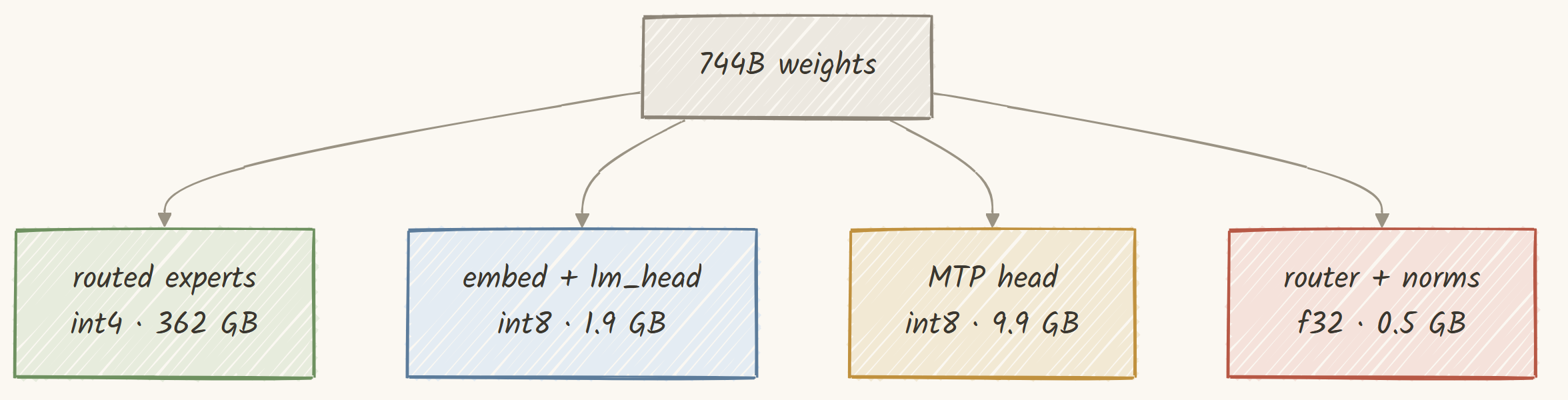
Not every tensor gets the same treatment, and choosing the right precision per tensor is where quality is won or lost. A small classifier decides the fate of each weight. The routed experts go to int4, because there are millions of them and they are the bulk of the model.
The embeddings and the output head stay at int8, because they are the input and output boundary and are sensitive. The router weights, the norms, and the biases stay in full float32, because they are small and they steer everything. And the multi token head and the sparse indexer are handled in their own passes.
def classify(name, n_layers, keep_mtp=False, keep_idx=False):
    if name.endswith("_scale_inv"): return "consumed"           # handled with its weight
    if name.endswith("e_score_correction_bias"): return "f32"   # router bias
    if name.endswith("mlp.gate.weight"): return "f32"           # the router itself
    if name.endswith("norm.weight") or name == "model.norm.weight": return "f32"
    if name in ("model.embed_tokens.weight", "lm_head.weight"): return "io"  # int8 boundary
    if ".mlp.experts." in name and name.endswith(".weight"): return "x"      # routed expert -> int4
    if name.endswith(".weight"): return "q"                     # attn / dense / shared -> int4
    return "f32"
There is one more thing the converter does that is worth calling out, and it is not about math at all, it is about disk. The FP8 checkpoint is 756 gigabytes. If you had to download all of it and then convert it, you would need more than a terabyte free. Instead the converter works one shard at a time.
It downloads one shard of about 5 gigabytes, converts it to int4, writes the result, and deletes the FP8 shard before moving on. The peak disk usage is never more than one shard plus the growing int4 output. So here is the command we run.
python tools/convert_fp8_to_int4.py --repo zai-org/GLM-5.2-FP8 --outdir /nvme/glm52_i4 \
    --ebits 4 --io-bits 8
How do we know the output is actually int4? We decode the bytes on disk. Our capture tool opened a converted shard and read the raw bytes of one expert's gate projection.
name: model.layers.0.mlp.gate_proj.weight
dtype: U8  shape(packed bytes): [37748736]  nbytes: 37748736
rows (from .qs): 12288  -> implied cols = nbytes*2/rows = 6144  => int4 (2 vals/byte) CONFIRMED
first 8 packed bytes: 87 78 77 89 b5 b8 77 77
decoded int4 values (nibble-8): [-1, 0, -1, 1, -3, 0, -1, -1] (low nibbles)
The packed data is 37,748,736 bytes, and the companion .qs tensor says there are 12,288 rows. Two values per byte means the implied number of columns is 37748736 * 2 / 12288, which is 6144, exactly the hidden size. So this is indeed two int4 values per byte.
The first byte, 0x87, decodes to a low nibble of 7 - 8 = -1 and a high nibble of 8 - 8 = 0, and you can see those first two decoded values are indeed negative 1 and 0. This is not a claim, it is the bytes.
The converter also has a self test for the FP8 dequant step, which round trips a random matrix through the 128 by 128 block scaling and reports the error.
[selftest fp8 block-dequant] mean relative error = 0.0226 (OK)A mean relative error of 2.26 percent for the FP8 block dequant is well within tolerance, and it passes. Now, if we step back and look at the whole model after conversion, we can ask where all the bytes went. Our census tool walked all 144 shards and classified every tensor by bit width and by role.
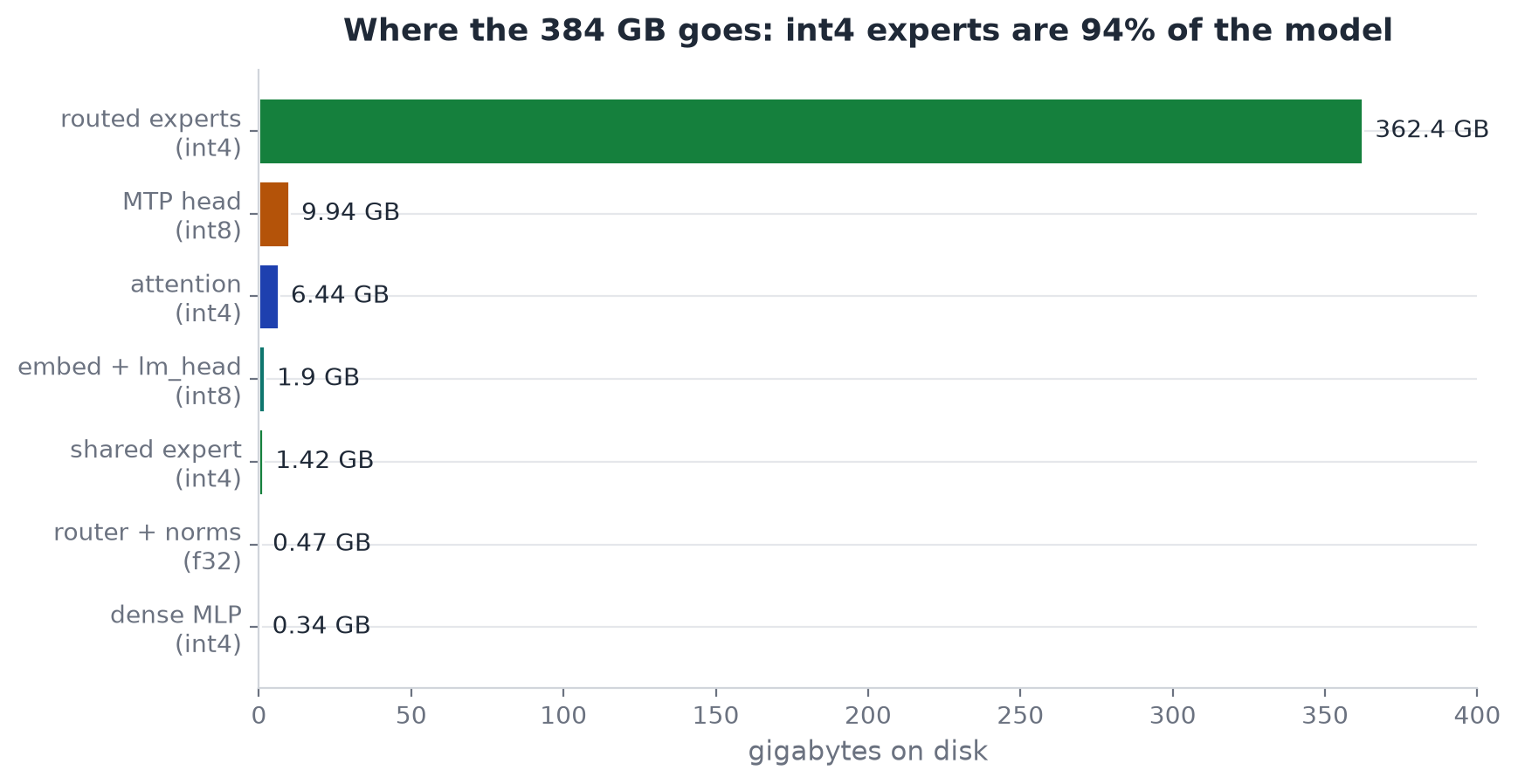
The routed experts, all int4, are 362 gigabytes, which is 94 percent of the model. The int8 parts, the multi token head and the input and output embeddings, are about 12 gigabytes. The full precision router weights, biases, and norms are under a gigabyte.
So when I say "we quantized the model to 4 bits," the census backs it up. Almost the entire mass of GLM 5.2 is now two values per byte, and the small sensitive parts kept their precision.
What Does int4 Actually Cost?
Quantizing to 4 bits is not free, and I do not want to wave that away. So let us measure the cost directly, using a tiny version of the exact architecture where we can compare the C engine token for token against a PyTorch reference.
The method is to quantize the weights to N bits, dequantize them back, run the engine, and see how many positions still match the reference. More bits should mean a closer match.

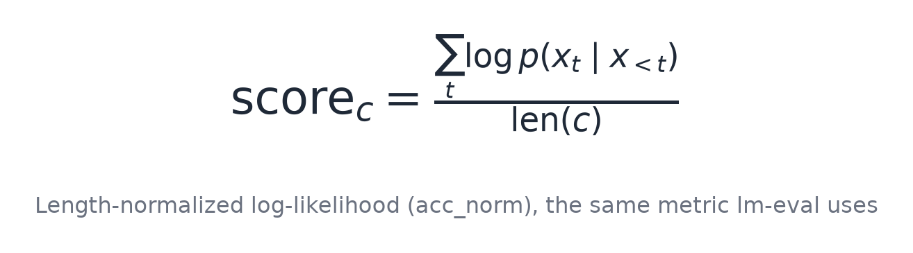
The way we score quality on the benchmarks is length normalized log likelihood, which is the same idea lm-eval uses. For each question, for each answer option, we sum the log probability the model assigns to that option and divide by its length in characters, and we pick the highest.
But the clearest single experiment is the bit width grid on the tiny oracle. We run teacher forcing over a 32 token sequence and count how many positions the engine predicts exactly like the PyTorch reference, at different bit widths for the experts and for the dense part. So let us run it at each of those bit widths and see.
== ./glm 64 16 16 ==   experts@16-bit dense@16-bit   ->  32/32 positions
== ./glm 64 8 8 ==     experts@8-bit  dense@8-bit    ->  30/32 positions
== ./glm 64 4 8 ==     experts@4-bit  dense@8-bit    ->  28/32 positions
== ./glm 64 4 4 ==     experts@4-bit  dense@4-bit    ->  9/32 positions
== ./glm 64 8 4 ==     experts@8-bit  dense@4-bit    ->  6/32 positions
== ./glm 64 2 2 ==     experts@2-bit  dense@2-bit    ->  1/32 positions
There is a genuine lesson hiding in these six lines, and it is not the one you might expect. Compare the two middle rows. When the experts are 4 bit and the dense path is 8 bit, we get 28 out of 32. When we flip it, experts at 8 bit and dense at 4 bit, we get only 6 out of 32.
The dense path, which is the attention and the shared experts, is far more sensitive to quantization than the routed experts are. This is exactly why our conversion keeps the embeddings, the output head, and the multi token head at int8 while pushing the experts to int4.
The bulk of the model can be aggressive, the sensitive parts cannot.
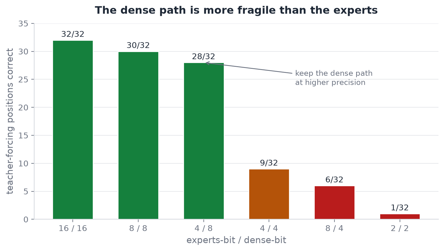
I should be honest about what this grid is and is not. It is a teacher forcing exactness probe on a tiny random model, so 9 out of 32 at 4 bit and 4 bit does not mean the full model is broken at int4. It is a sensitivity measurement, not a quality benchmark.
The int4 model answers questions correctly, as we will see when we run actual conversations. What the grid tells us is the relative fragility of the parts, and that guided the bit policy.
There is one more check I care about, because it is the thing that lets the offline converter and the runtime agree. We compared two paths. In path A, the C engine reads the tiny oracle's full precision weights and quantizes them to int4 itself at runtime.
In path B, the Python converter produces the int4 container and the C engine reads it verbatim.
A: oracle full weights, C engine runtime-quantizes to int4 (pack_int4):
   PREFILL (teacher-forcing) C vs oracle: 9/32 positions
B: python-converter int4 container, C engine reads it verbatim:
   PREFILL (teacher-forcing) C vs oracle: 9/32 positions
(identical X/32 => python np.rint quantizer == C lrintf pack_int4)
Both give 9 out of 32, identically. That identical result is the proof that the NumPy np.rint path and the C lrintf path pack the same bytes. If they disagreed by even one nibble, these numbers would drift apart. So we can convert offline in Python and run in C and trust that the model is bit for bit the same.
That trust is what the whole pipeline stands on.
Loading Weights by Streaming, Not Loading
Now that we have an int4 container on disk, we need to read it, and how we read it is the difference between a model that fits and one that does not. The naive approach is to memory map the whole thing and let the operating system page it in. That works, but it has a trap.
Once a page is touched it stays resident in the process, so your resident memory creeps up toward the full model size, and the whole point was to keep resident memory small. We do the opposite. We read exactly the bytes we need with pread, and we tell the kernel to drop those pages right after.

The first job is finding a tensor quickly. GLM 5.2 has about 120,000 tensors across 144 shard files, because each of the 19,456 experts has three matrices and each matrix has its scale companion. A linear scan of that list per tensor lookup cost tens of seconds per token on the first full run, which is absurd.
So we build a hash index once at startup and look tensors up by name in constant time.
/* Index every tensor in every shard. Names go into an open-addressing hash map,
 * because GLM has ~120k tensors and a linear scan cost tens of seconds/token. */
typedef struct {
    char *name; int fd; int64_t off; int64_t nbytes; int dtype; int64_t numel;
} st_tensor;

static st_tensor *st_find(shards *S, const char *name) {
    uint64_t h = st_hash(name) & (S->hcap - 1);
    while (S->hidx[h] >= 0) {
        st_tensor *t = &S->t[S->hidx[h]];
        if (!strcmp(t->name, name)) return t;
        h = (h + 1) & (S->hcap - 1);
    }
    return NULL;
}
Each st_tensor records which file descriptor holds it, the byte offset inside that file, the byte count, and the data type. The hash is a plain FNV-1a over the tensor name, and we use open addressing so lookups never chase pointers.
That one change took tensor lookup from a measurable fraction of every token down to nothing.
Now the read itself. Here is the function that reads a tensor into a caller supplied float32 buffer, converting from bfloat16 or float16 if needed, and, crucially, dropping the pages afterward when we ask it to.
/* Read a tensor into a float32 buffer. drop=1 advises the kernel to discard the
 * pages after the read (for streaming experts), so peak RSS stays dense + cache. */
static int64_t st_read_f32(shards *S, const char *name, float *out, int drop) {
    st_tensor *t = st_find(S, name);
    if (!t) { fprintf(stderr, "missing tensor: %s\n", name); exit(1); }
    void *raw = malloc(t->nbytes);
    if (pread(t->fd, raw, t->nbytes, t->off) != t->nbytes) { perror("pread data"); exit(1); }
    if (t->dtype == 2)      memcpy(out, raw, t->nbytes);                       /* f32 */
    else if (t->dtype == 0) { uint16_t *p = raw; for (int64_t i = 0; i < t->numel; i++) out[i] = bf16_to_f32(p[i]); }
    else                    { uint16_t *p = raw; for (int64_t i = 0; i < t->numel; i++) out[i] = f16_to_f32(p[i]); }
    free(raw);
    if (drop) posix_fadvise(t->fd, t->off, t->nbytes, POSIX_FADV_DONTNEED);    /* drop the pages */
    return t->numel;
}
The posix_fadvise call with POSIX_FADV_DONTNEED is the important line here. After we have read an expert and copied its bytes into our own slab, we tell the kernel it can forget those file pages.
This is what keeps our peak resident memory equal to the dense part plus whatever cache we choose, instead of the whole model.
For weights that are already quantized in our container, there is a sibling function st_read_raw that reads the raw bytes with no dtype conversion at all, because int4 and int8 data does not need converting.
There is also a second file descriptor open on each shard, opened with O_DIRECT, that bypasses the page cache entirely. On some disks the buffered read path serializes and chokes, and the direct path is faster. We keep both and pick per situation. Now, how fast can this disk actually feed us?
Our I/O benchmark reads expert sized 19 megabyte blocks at random, the exact access pattern the engine has, with several threads.
buffered x8 threads: 64 reads x 19MB = 1.3 GB in 0.40s -> 3.22 GB/s (6.2 ms/block)
O_DIRECT x8 threads: 64 reads x 19MB = 1.3 GB in 0.31s -> 4.13 GB/s (4.8 ms/block)
So the cold disk ceiling for our access pattern is about 4 gigabytes per second with direct reads, and each 19 megabyte expert takes about 5 milliseconds to pull. That number is the budget for everything downstream.
If we have to read all 8 experts per layer across 75 layers cold, that is 600 reads, roughly 11 gigabytes, and even at 4 gigabytes per second that is seconds per token. The whole tiering system exists to avoid paying that cold price. Here is the full read sweep across block sizes and thread counts.
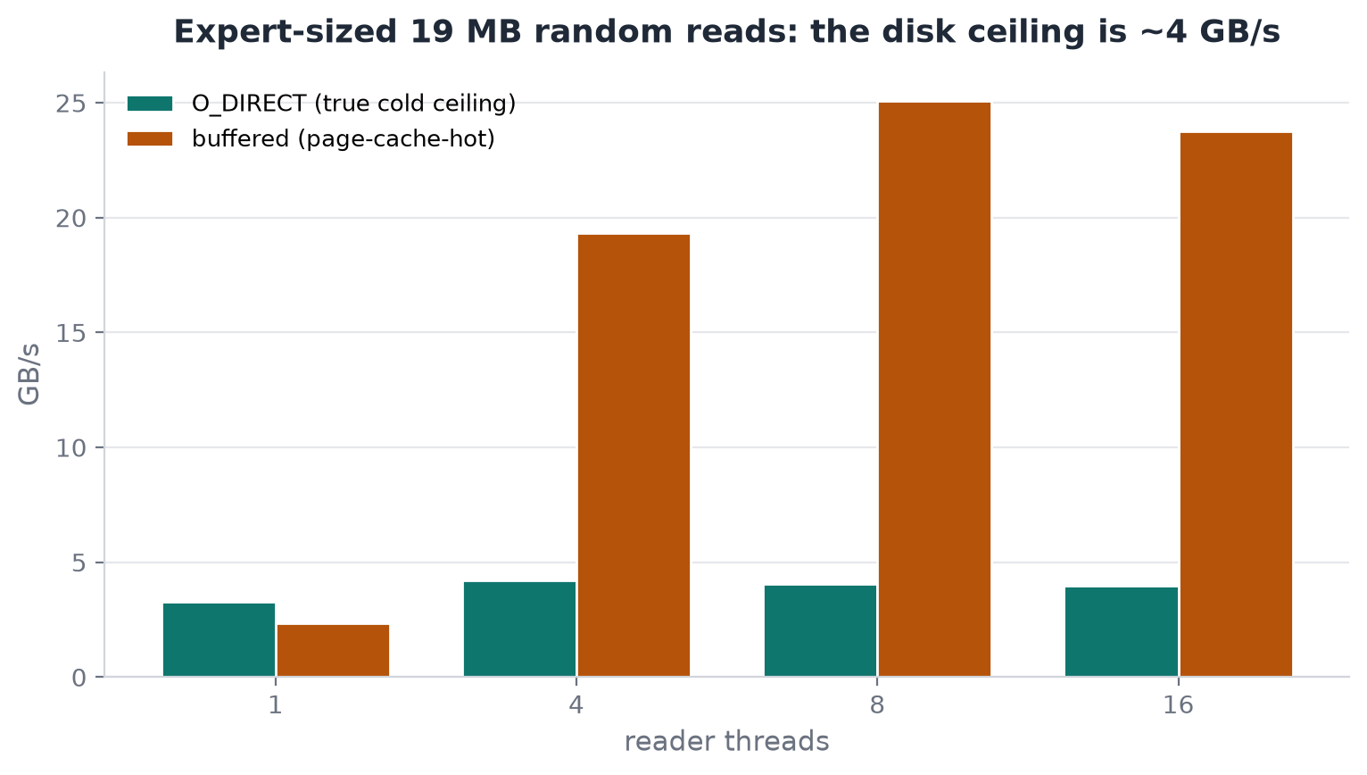
Notice the buffered bars tower over the direct ones. That is not the disk getting faster, that is the page cache returning bytes we already read. It is a genuine speedup and we will exploit it, but it is honest to label it as cache, not disk. The true cold ceiling is the teal bars, around 4 gigabytes per second.
Attention: Multi head Latent Attention With a Tiny KV Cache
Attention is where GLM 5.2 does something that helps us enormously. It does not store a full key and value for every head at every position. It uses Multi head Latent Attention, which keeps a single compressed latent per token and reconstructs the keys and values from it on the fly.
This is the difference between a KV cache that fits in memory and one that does not, because GLM 5.2 has 64 attention heads and no grouped query attention to shrink them.
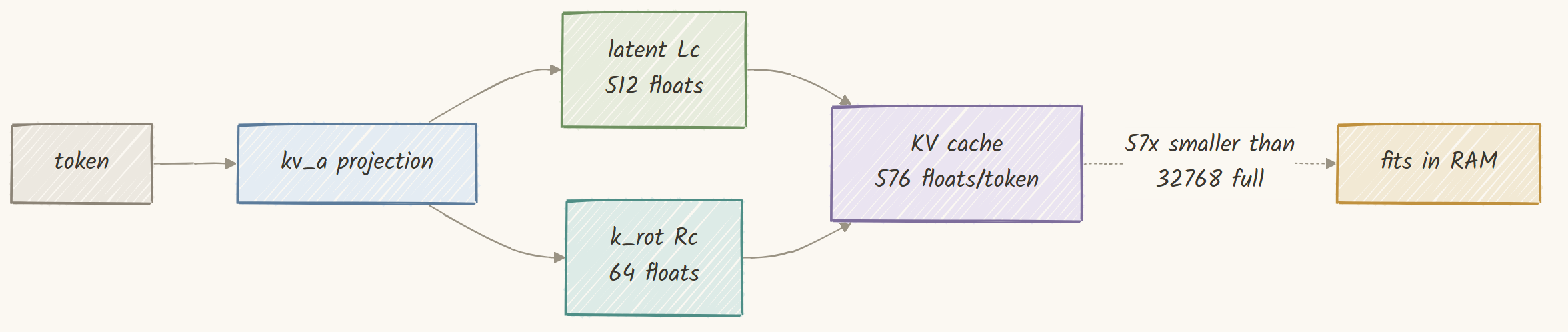
Let me make the saving concrete. A full key plus value for all 64 heads would be 64 * (256 + 256), which is 32,768 floats per token. What we actually store is the compressed latent of kv_lora_rank 512 floats plus the rotary part qk_rope_head_dim of 64 floats, which is 576 floats per token.
That is about 57 times smaller.

Here is the cache state. Notice it only holds the latent Lc and the rotary key Rc per layer, nothing else.
/* The MLA compressed KV cache: per token we keep only the normalized latent
 * Lc [kv_lora] and the rotary key Rc [qk_rope], which is 576 vs 32768 floats
 * per token. k_nope and value are reconstructed on the fly from kv_b. */
typedef struct {
    float **Lc, **Rc, **Ic;
    int *kv_start, max_t;
    int disk_nrec;
    char disk_path[2048];
} KVState;
During decoding, when we are generating one token at a time, we never actually rebuild the full keys and values for the whole context. There is a linear algebra identity, sometimes called weight absorption, that lets the query absorb the key up projection so we can score against the small latents directly.
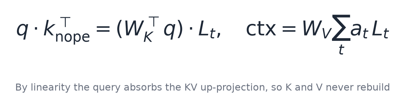
By linearity, the dot product of the query with the reconstructed key equals the dot product of an absorbed query with the stored latent.
So we fold the key up projection into the query once, then every score is just a dot product against a 512 dimensional latent, and the context is a weighted sum of latents projected back out at the end.

Here is the main part of that decode path.
/* Weight absorption for decode (small S). By linearity q . k_nope = (W_K^T q) . L_t,
 * so the query "absorbs" kv_b once, then every score is a dot against the latent.
 * Cost per step is O(T * kv_lora) instead of rebuilding k/v for every token. */
#pragma omp parallel for collapse(2) schedule(static)
for (int s = 0; s < S; s++) for (int h = 0; h < H; h++) {
    const float *qp = Q + (int64_t)s*H*qh + (int64_t)h*qh;
    const float *qr = qp + c->qk_nope;                      /* the rotary part */
    float qabs[512]; memset(qabs, 0, kvl * sizeof(float));
    for (int d = 0; d < c->qk_nope; d++)                    /* absorb kv_b into the query */
        qt_addrow(&l->kv_b, rbase + d, qp[d], qabs);
    float *sc = sc_all + (int64_t)omp_get_thread_num() * sc_cap;
    for (int jj = 0; jj < nt; jj++) {                       /* score vs each latent */
        const float *Lt = kv_row(ks->Lc[layer], st0 + jj, kvl);
        const float *kr = kv_row(ks->Rc[layer], st0 + jj, c->qk_rope);
        float a = 0; for (int i = 0; i < kvl; i++) a += qabs[i] * Lt[i];
        for (int d = 0; d < c->qk_rope; d++) a += qr[d] * kr[d];
        sc[jj] = a * c->attn_scale;
    }
    softmax(sc, nt);
    float clat[512]; memset(clat, 0, kvl * sizeof(float));  /* pool the latent */
    for (int jj = 0; jj < nt; jj++) {
        const float *Lt = kv_row(ks->Lc[layer], st0 + jj, kvl);
        float a = sc[jj]; for (int i = 0; i < kvl; i++) clat[i] += a * Lt[i];
    }
    qt_matvec_rows(&l->kv_b, rbase + r0v, vh, clat, ctx + ((int64_t)s*H + h)*vh);
}
There is a lot of detail here, and the comments carry it, but the shape is what I want you to take away. We absorb the up projection into the query, we score against small latents, we softmax, we pool the latents, and we project once at the end. No per token key and value reconstruction during decode.
For the prefill of a long prompt, where we process many tokens at once, we do reconstruct the keys and values in one batched matmul, because there it is cheaper to do it in bulk. The engine chooses between the two automatically based on how many tokens are in flight.
Is the absorbed path truly equal to the explicit one? We checked, on the tiny oracle, running both and comparing tokens.
== ABSORB=1 (absorbed low-rank MLA) ==
GLM C engine : 207 187 119 103 103 103 103 103 119 34 ...
== ABSORB=0 (explicit K/V reconstruction) ==
GLM C engine : 207 187 119 103 103 103 103 103 119 34 ...
Identical token streams. The absorption is a reformulation, not an approximation. Because the KV cache is so small, we can also afford to write it to disk and reopen a conversation warm. The compressed cache costs about 182 kilobytes per token, and here is a persisted cache file on disk.
file: /nvme/glm52_i4/.glm_kv
-rw-rw-r-- 1 ubuntu ubuntu 45108756 ... .glm_kv
That is a 45 megabyte cache holding an actual conversation. The reason this matters is that re prefilling a reopened chat on our slow disk would cost minutes, and reloading the cache costs milliseconds. We tested it by generating in one process, killing it, and resuming in a completely new process.
===== RUN 1: fresh prompt, generate, persist KV =====
One Two Three Four Five Six Seven Eight Nine Ten Eleven Twelve Thirteen Fourteen Fifteen Sixteen Se
===== RUN 2: NEW process reopens .glm_kv, continues, no re-prefill =====
[KV] resumed conversation from disk: 57 tokens in 0.0s (no re-prefill)
Seventeen Eighteen Nineteen Twenty
The second process picked up exactly where the first left off, counting from seventeen, and it resumed 57 tokens in zero seconds with no re prefill. The conversation reopened warm.
The Lightning Indexer: Sparse Attention When It Helps
GLM 5.2 has one more attention feature, and it only turns on when it is needed. It is a sparse attention indexer, sometimes called a lightning indexer. On long contexts, instead of attending to every past token, the model attends only to the most relevant ones.
The indexer is a small scoring network that picks which past keys are worth attending to.

For each query, the indexer computes a small query and small keys, scores every past position, and keeps the top index_topk, which is 2048, of them. The scoring uses a rectified dot product per head and then a weighted sum across heads.
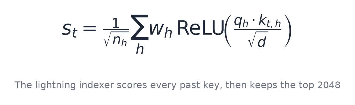
Here is the scoring loop from the engine. Notice the if (d0 > 0), which is the ReLU, and the top k selection by sorting the scores and taking a threshold.
/* For each query, score every past key with a ReLU'd per-head dot product,
 * weight and sum across heads, then keep the top index_topk positions. */
float wsc = 1.f / sqrtf((float)nh), rs = 1.f / sqrtf((float)hd);
float *isc = falloc(nk);
for (int t = 0; t < nk; t++) {
    const float *kt = kv_row(ks->Ic[layer], t, hd);
    float a = 0;
    for (int h = 0; h < nh; h++) { const float *qhp = qi + (int64_t)h*hd;
        float d0 = 0; for (int i = 0; i < hd; i++) d0 += qhp[i] * kt[i];
        d0 *= rs; if (d0 > 0) a += w32[h] * d0;        /* ReLU on the score, then weight */
    }
    isc[t] = a * wsc;
}
/* top-keep: threshold via a descending sort, then scan in position order */
float *tmp = falloc(nk); memcpy(tmp, isc, nk * sizeof(float));
qsort(tmp, nk, sizeof(float), cmp_fdesc);
float thr = tmp[keep - 1];
int *dst = m->dsa_sel + (int64_t)s * dtopk, nd = 0;
for (int t = 0; t < nk && nd < keep; t++) if (isc[t] > thr) dst[nd++] = t;
The important property for correctness is that the indexer is a no operation when the context is shorter than index_topk. If there are fewer than 2048 past keys, selecting the top 2048 selects all of them, and the attention is exactly the same dense attention we would have done anyway.
So short prompts are bit for bit identical whether the indexer is on or off. We confirmed that by running with the indexer forced on, off, and default, and diffing the generated text.
=== DSA_FORCE=1 vs default ===   generated text: identical (only the timing banner differs)
=== DSA=0 vs default ===         generated text: identical (only the timing banner differs)
The only differences between the runs were the load time banners. The generated tokens were the same. That is the behavior we want. The sparse path only changes anything once the context is long enough to need it, and even then it is the model's own designed mechanism, not an approximation we invented.
MoE Routing and Expert Dispatch
Now the main computation, the Mixture of Experts layer. For each token the router scores all 256 experts, we pick the top 8, and we run those experts and add their weighted outputs.
GLM 5.2 uses a sigmoid router with a correction bias, and one detail that is easy to get wrong is which number decides selection and which number becomes the weight.

The router applies a sigmoid to each expert's logit. It then adds a per expert correction bias, and it selects the top 8 by that biased value. But the weight it keeps for each selected expert is the plain sigmoid, without the bias. The bias steers selection, the sigmoid is the weight.
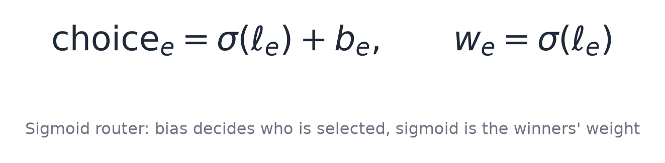
Here is that routing logic from the engine.
/* Phase A: route every position. sigmoid(logit) + bias picks the top-K,
 * but the weight kept is sigmoid(logit) of the winners, not the biased value. */
for (int s = 0; s < S; s++) {
    const float *xs = x + (int64_t)s * D;
    matmul(logit, xs, l->router, 1, D, E);
    for (int e = 0; e < E; e++) { logit[e] = sigmoidf(logit[e]); choice[e] = logit[e] + l->router_bias[e]; }
    int *idx = idxs + (int64_t)s*K; float *w = ws + (int64_t)s*K;
    for (int kk = 0; kk < K; kk++) {                        /* top-K by choice */
        int best = -1; float bv = -1e30f;
        for (int e = 0; e < E; e++) { int tk = 0; for (int j = 0; j < kk; j++) if (idx[j] == e) { tk = 1; break; }
            if (!tk && choice[e] > bv) { bv = choice[e]; best = e; } }
        idx[kk] = best; w[kk] = logit[best];               /* weight = sigmoid, not choice */
    }
    for (int kk = 0; kk < K; kk++) {                        /* track usage for the cache */
        m->eusage[layer][idx[kk]]++;
        if (m->eheat[layer][idx[kk]] < UINT32_MAX) m->eheat[layer][idx[kk]]++;
        m->elast[layer][idx[kk]] = ++m->eaccess_clock;
    }
    for (int kk = 0; kk < K; kk++) w[kk] *= c->routed_scale;
}
Every selection also bumps three counters, eusage, eheat, and elast. Those are the persistent usage, the recent heat, and the recency clock, and they are the signals that drive the whole tiering system in the next section. Routing is not just picking experts, it is also learning which experts are hot.
When we process more than one token at a time, during prefill or when verifying speculative drafts, we do something that saves a lot of disk. We take the union of the unique experts across all positions in the batch, load each unique expert exactly once, and apply it to every position that routed to it.
The weights are read from disk once, not once per token.
/* Phase B: union of unique experts across the batch. Each unique expert is
 * loaded once and applied to every position that routed to it. */
int *uniq = malloc((size_t)E * sizeof(int)); int nu = 0;
unsigned char seen[E]; memset(seen, 0, (size_t)E);
for (int s = 0; s < S; s++) for (int kk = 0; kk < keff[s]; kk++) {
    int e = idxs[(int64_t)s*K + kk];
    if (!seen[e]) { seen[e] = 1; uniq[nu++] = e; }
}
Once an expert is in hand, the computation is a SwiGLU. We run the gate and up projections, apply the sigmoid linear unit to the gate and multiply by the up, then run the down projection.
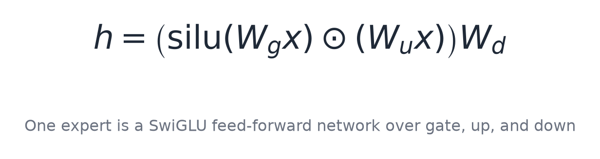
/* Each expert: gate and up projections, silu(gate) * up, then down projection,
 * scaled by the routing weight and added to the output. */
expert_gate_up(gg, uu, xg, &e->g, &e->u, nr);              /* gate and up */
for (int64_t z = 0; z < (int64_t)nr*I; z++) gg[z] = siluf(gg[z]) * uu[z];   /* silu(g) * u */
matmul_qt(hh, gg, &e->d, nr);                              /* down */
for (int r = 0; r < nr; r++) {
    float *os = out + (int64_t)rows[r]*D, wgt = rw[r], *hr = hh + (int64_t)r*D;
    for (int d = 0; d < D; d++) os[d] += wgt * hr[d];
}
There is also a shared expert, which runs for every token regardless of routing, and its output is added to every position. Now, does the routing actually concentrate on a few experts? If it did not, the caching later would be pointless. We captured the routing histogram from a run and looked at the hottest experts.
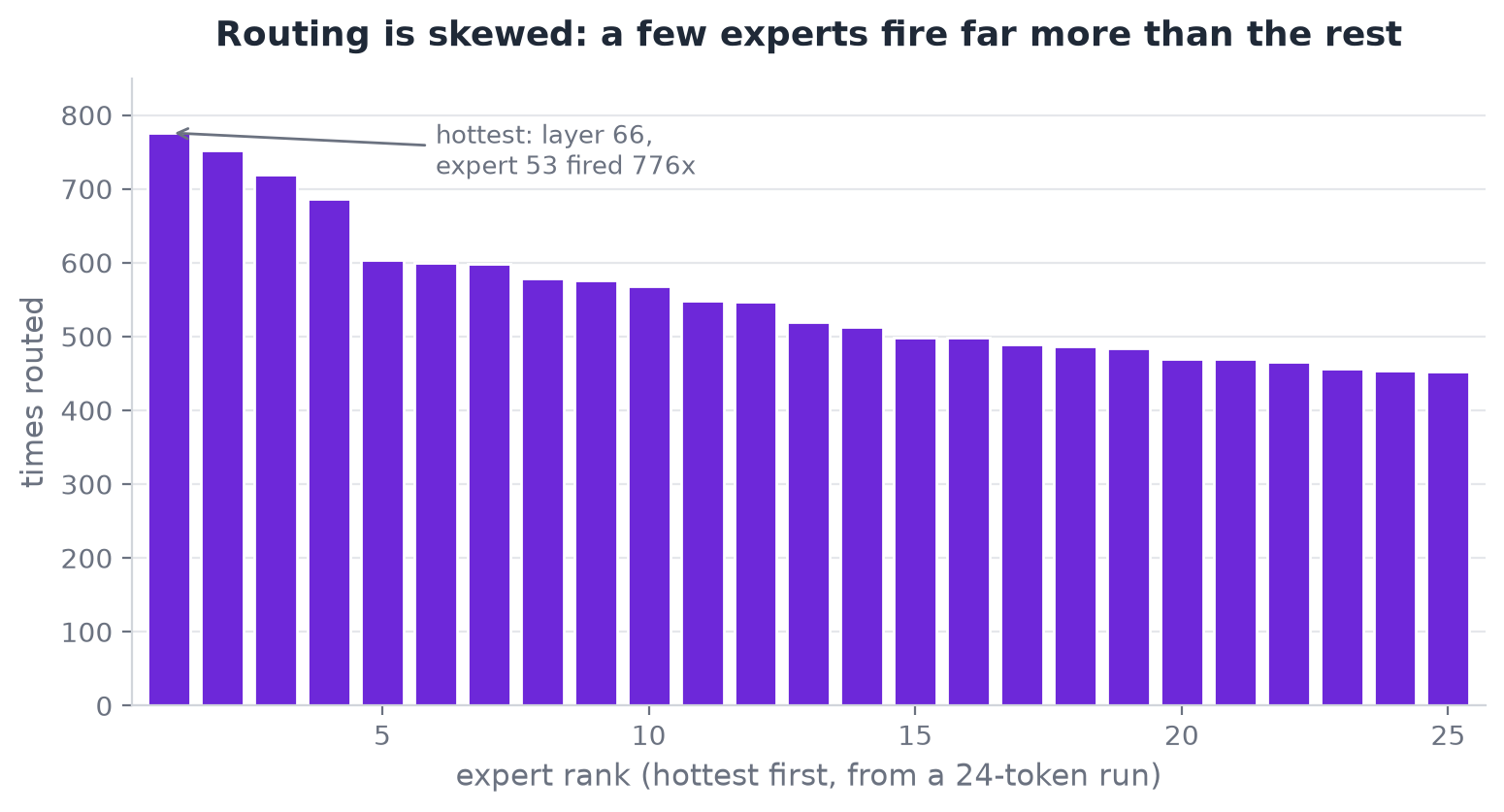
The distribution is heavily skewed. The hottest expert, at layer 66, expert 53, fired 776 times in a short run, and the counts fall off from there. This skew is the reason the tiering works.
If we keep the hot head of the distribution resident, we serve most requests from memory and only occasionally reach for a cold expert on disk. Routing tells us which experts to keep close.
The Kernels: Integer Dot Products
Underneath all of this are the matrix multiplies, and they are where the CPU time goes. We have a small family of them. A plain float matmul, an int8 one that dequantizes on use, an int4 one, and an int2 one.
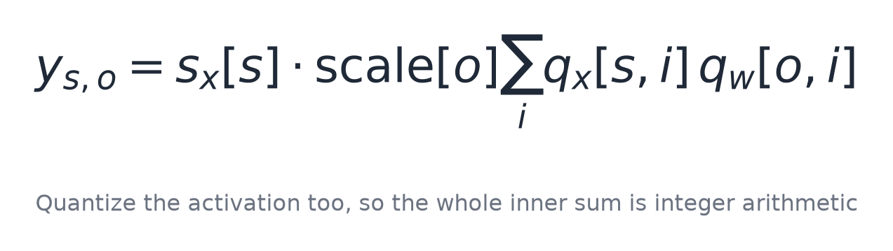
But the interesting kernels are the integer ones, where instead of dequantizing the weights to float in the hot loop, we quantize the activation to int8 as well and do the entire inner product in integer arithmetic.
The idea is that if both the activation and the weight are small integers, the dot product is a sum of integer products, and we multiply by the two scales only at the very end.
First we quantize an activation row to int8, the same symmetric absmax we use everywhere.
/* Quantize an activation row to int8 (absmax / 127), Q8_0 style, returning the scale. */
static inline float qrow_i8(const float *x, int8_t *q, int I) {
    float amax = 0; for (int i = 0; i < I; i++) { float a = fabsf(x[i]); if (a > amax) amax = a; }
    float s = amax / 127.f; if (s < 1e-12f) s = 1e-12f; float inv = 1.f / s;
    for (int i = 0; i < I; i++) q[i] = (int8_t)lrintf(x[i] * inv);
    return s;
}
Then the integer dot product itself. On AVX2 we have a nice sign trick. There is no instruction to multiply two signed bytes and accumulate, but there is one to multiply an unsigned byte by a signed byte.
So we take the absolute value of the weight, which makes it unsigned, and we fold the weight's sign into the activation. The result is the same, and it fits the instruction we have.
/* int8 . int8 dot with the sign trick: |w| is unsigned, sign(w) is folded into x,
 * so maddubs (unsigned * signed) works. Safe: each pair <= 128*127*2 = 32512 < 32767,
 * so the 16-bit intermediates never saturate up to I = 16384. */
static inline int32_t dot_i8i8(const int8_t *w, const int8_t *x, int I) {
    int32_t sum = 0; int i = 0;
#if defined(__AVX2__)
    __m256i acc = _mm256_setzero_si256(); const __m256i
    for (; i + 32 <= I; i += 32) {
        __m256i wv = _mm256_loadu_si256((const __m256i*)(w + i));
        __m256i xv = _mm256_loadu_si256((const __m256i*)(x + i));
        __m256i p = _mm256_maddubs_epi16(_mm256_sign_epi8(wv, wv), _mm256_sign_epi8(xv, wv));
        acc = _mm256_add_epi32(acc, _mm256_madd_epi16(p, ones));
    }
    sum = hsum256_i32(acc);
#endif
    for (; i < I; i++) sum += (int32_t)w[i] * x[i];        /* scalar tail */
    return sum;
}
The comment carries the safety argument, and it is worth reading because it is the kind of thing that silently corrupts output if you get it wrong. Each product of two bytes is at most 128 times 127, and we add two of them into a 16 bit lane, giving at most 32,512, which is under the 32,767 that would overflow.
So the intermediate never saturates for input widths up to 16,384, which covers our matrices. There is a matching kernel for int4 weights that unpacks the nibbles to int8 on the fly and then does the same trick.
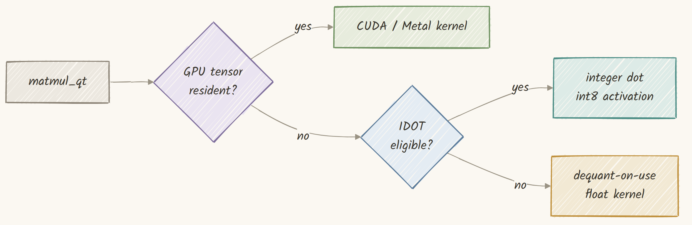
All of these kernels sit behind one dispatcher, matmul_qt, which is the single place that decides how to run a quantized matmul. It tries the GPU first if the tensor is resident there, then the integer path if it is eligible, then falls back to the float kernels.
/* The one dispatcher for a quantized matmul. Try the GPU, then the integer
 * kernels (int8 always; int4 above a per-ISA threshold), then float. */
static void matmul_qt(float *y, const float *x, QT *w, int S) {
#ifdef GLM_CUDA
    if (g_cuda_enabled && w->cuda_eligible && !w->cuda_failed && !omp_in_parallel()) {
        if (glm_cuda_matmul(&w->cuda, y, x, weights, w->s, w->fmt, S, w->I, w->O, w->cuda_device)) return;
    }
#endif
    if (w->fmt == 0) { matmul(y, x, w->qf, S, w->I, w->O); return; }
    if (g_idot && (w->fmt == 1 || (w->fmt == 2 && S >= g_i4s))) {   /* integer path */
        int I = w->I; int8_t *xq; float *sx;
        quant_scratch((size_t)S*I, (size_t)S, &xq, &sx);
        for (int s = 0; s < S; s++) sx[s] = qrow_i8(x + (int64_t)s*I, xq + (int64_t)s*I, I);
        if (w->fmt == 1) matmul_q_idot(y, xq, sx, w->q8, w->s, S, I, w->O);
        else matmul_i4_idot(y, xq, sx, w->q4, w->s, S, I, w->O);
        return;
    }
    if (w->fmt == 1) matmul_q(y, x, w->q8, w->s, S, w->I, w->O);    /* float fallbacks */
    else if (w->fmt == 3) matmul_i2(y, x, w->q4, w->s, S, w->I, w->O);
    else matmul_i4(y, x, w->q4, w->s, S, w->I, w->O);
}
Because integer arithmetic has no rounding, the SIMD kernels must produce exactly the same integer sum as a plain C loop. We test that, and it is one of the tests that passed earlier.
----- test_idot ----- idot kernel exactness (avx2): okThat ok means the AVX2 integer dot product returns bit identical results to a scalar reference across odd sizes and edge cases, including the tricky value negative 128. When we profile a decode, these kernels are exactly where the time goes.
matmul_i4_pair._omp_fn.0    8.87%
matmul_i4_idot._omp_fn.0    8.33%
matmul_i4._omp_fn.0         4.99%
matmul_q_idot._omp_fn.0     2.34%
attention_rows._omp_fn.1    1.79%
The named hot symbols are all our int4 matmul variants. Now, there is an honest caveat about the integer path, and I want to state it plainly. Quantizing the activation to int8 adds a tiny amount of noise, about 0.3 percent RMS per matmul, and that can occasionally flip a token compared to the exact float path.
We measured it directly.
=== IDOT=1 (int8 activation) ===  A mutex (mutual exclusion) is
=== IDOT=0 (f32 reference)   ===  A mutex (mutual exclusion object)
Same prompt, and the two paths diverge by one word after a few tokens. Both answers are correct, but they are not bit identical. This is the trade we make for speed on the CPU, and we expose a switch to turn the integer path off when you need exact reproducibility.
It is the kind of thing I would rather tell you about than hide.
The Tiering System
Everything so far has been building toward this. We have a 370 gigabyte pile of experts on disk, a fast but not infinite disk, and a skewed routing d